If you wish to interactively try the task, select parameters for the task below. Leave the settings at the defaults to be randomly assigned to a condition. The task code is in javascript and will run locally on your computer; no data is sent anywhere. At the end, you will have the option to save your data.
A short video showing the task can be found under inst/manuscript/img/santa_task_example.mp4 (click ‘View raw’ to download).
Users of the MoreyHoekstra2019 R package can also load a version of the experimental task:
Task details
In a nutshell, the main task is to determine the sign of an effect, if it is nonzero.
Effect sizes
Participants were randomly assigned to one of eight effect size conditions, each with a unique toy name. The sign of the effect was then also randomly assigned (each with 50% probability). Because we were particularly interested in false positives, we assigned participants to the “no effect” condition with greater probability.
#> `summarise()` ungrouping output (override with `.groups` argument)| Toy name | Hidden effect size (δ) | Probability |
|---|---|---|
| whizbang balls | 0.00 | 0.25 |
| constructo bricks | 0.10 | 0.11 |
| rainbow clickers | 0.19 | 0.11 |
| doodle noodles | 0.30 | 0.11 |
| singing bling rings | 0.43 | 0.11 |
| brahma buddies | 0.60 | 0.11 |
| magic colorclay | 0.79 | 0.11 |
| moon-candy makers | 1.00 | 0.11 |
In the task, participants could sample test statistics at will from either a null distribution (\(\delta=0\); called “random shuffle reports”) or the “experimental” distribution (with their assigned effect size).
Sample sizes
The participants could choose the sample size per “team”, but the number was hidden from them. The sample size slider has 20 increments, corresponding to team sizes of 10 to 200. The table below shows the sample sizes, which increased non-linearly as a function of the increment. To induce a resource cost to experimentation, the time a participant had to wait for an experimental sample was proportional to the team size. Null samples were instantaneous.
#> `summarise()` ungrouping output (override with `.groups` argument)| n index | n | Time (s) |
|---|---|---|
| 1 | 10 | 1 |
| 2 | 12 | 2 |
| 3 | 14 | 2 |
| 4 | 16 | 2 |
| 5 | 19 | 2 |
| 6 | 22 | 3 |
| 7 | 26 | 3 |
| 8 | 30 | 3 |
| 9 | 35 | 4 |
| 10 | 41 | 5 |
| 11 | 48 | 5 |
| 12 | 57 | 6 |
| 13 | 66 | 7 |
| 14 | 78 | 8 |
| 15 | 91 | 10 |
| 16 | 106 | 11 |
| 17 | 125 | 13 |
| 18 | 146 | 15 |
| 19 | 171 | 18 |
| 20 | 200 | 20 |
When a participant generated a sample, they were generating a test statistic. Hidden from the participant, the underlying test statistic was simply a \(Z\) statistic, sampled from the appropriate distribution:
\[ Z \sim \mbox{Normal}(\delta\sqrt{n/2}, 1) \]
where \(n\) was determined by the sample size slider selection, and \(\delta\) by the participant’s randomly assigned effect size (or \(\delta=0\) if they are drawing null samples).
However, the participant was not shown the \(Z\) statistic.
Evidence power
The \(Z\) statistic was transformed by the following equation, not known to the participant:
\[ x = \mbox{sgn}(Z)\left[1 - \left(1 - F_{\chi_1^2}\left(Z^2\right)\right)^{\frac{1}{q}}\right] \]
The value \(x\) gives the location on the experimental “interface” and the color (from left, -1 to right, or 1). The power \(q\) was randomly assigned to the participant (3 or 7, with equal probability).
The value \(x\) is a monotone transformation of the \(Z\) statistic, and hence contains the same information. The value \(q\)—called the “evidence power”—only changes the visual effect of the samples. When \(q=7\), the visual sampling distribution is narrower on the task interface; when \(q=3\), it is wider.
The figure below shows the distributions of the visual evidence (\(x\)) when \(\delta=0.19\) (“rainbow clickers”). Each distribution is a sample size; with increasing sample size, the visual distibution of the test statistic moves further to the right. More extreme values are expected as the sample size increases.
The figure below is for \(q=7\), the narrow transformation.

Evidence power 7, distributions
When the evidence power is \(q=3\), all distributions is visually much further to the right.

Evidence power 3, distributions
The null sampling distributions (the distribution of the “random shuffle reports”) are affected by the same transformation. The sampling distribution for the “wide” evidence power is visually wider than the narrow one.
We can show see the relative visual spread of the sampling distributions by adding the implied \(p\) values to the interface. The participant, of course, would not see these. The figure below shows the implied \(p\) values from the narrow null evidence distribution:
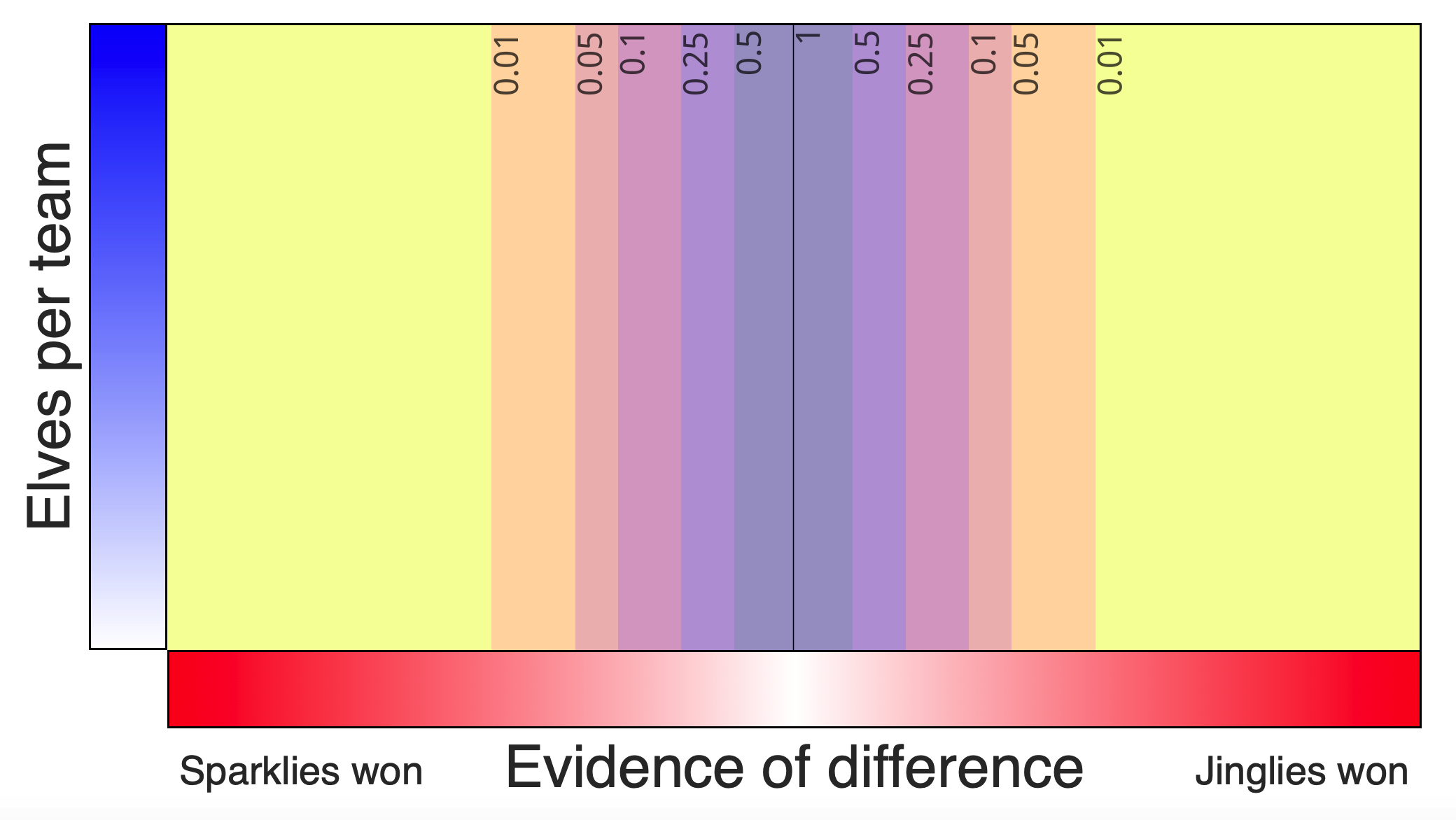
Evidence power 7, p values
And the wide null evidence distribution:
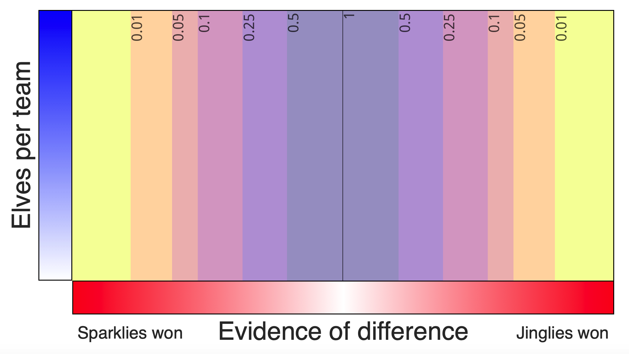
Evidence power 3, p values
These distributions must be discovered by the participant by sampling the random shuffle reports. To better see the effect of the evidence power maipulation, we have created an animation that shows how two hypothetical participants who got the same underlying data, but were randomly assigned to different evidence power conditions, would see the experiment. The top shows the narrow evidence power; the bottom, the wide evidence power. The \(p\) values are for reference and would not be shown to the participant.
Potential strategies
When they are ready, participants must decide which of the two teams was faster based on the data they collected. There are several strategies one might deploy:
- Null sampling distribution: Compare “experiments” to their respective null samples (“random shuffle reports”) to determine if results as extreme would be unlikely. Under this strategy, “extremeness” is scaled by the sampling distribution. This is a significance testing stragegy.
- Sign test: Count the number of experiments on each side to see if, on balance, they favor one side. This is a significance testing strategy, but a weak one (it throws away a lot of information).
- Visual extremeness: Base the decision on visual extremeness. This is an invalid strategy, but one that might be deployed by someone who did not understand significance testing. Both color and horizontal distance are the most salient features of the display if someone does not know how to use the random shuffle reports.
Hypotheses
The manipulation of evidence power is designed to determine whether people are using the salient visual cues (color and distance) or the valid significance-testing information (the null sampling distribution) to perform the task.
If participants are using a significance testing strategy, the probability that one decides in favor of a team should be determined by the extremeness of the evidence relative to the null sampling distribution. Thus, visual extremeness will matter much more to participants in the narrow condition than in the wide.
If participants use an invalid distance/color-based strategy, the probability that one decides in favor of a team should be determined by the visual extremeness of the evidence. When aligned on the null sampling distribution, participants will be much more willing to decide in favor of a difference in the wide condition.